Tag Archive: regression


🤔 What is it?

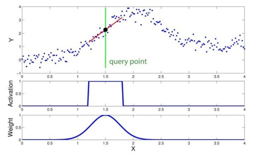
LWR is a non-parametric regression technique used in machine learning to model the relationship between a dependent variable and one or more independent variables. It is ideal for non-linear relationship modeling between variables as it does not assume a specific functional form. LWR is memory-based, storing the entire training dataset and making predictions based on the closest observations to the new data point. Model parameters are computed individually for each new data point, allowing for more customized and accurate predictions. It has applications in finance, economics, ecology, engineering, and can be used for time-series forecasting, data smoothing, and data imputation.

🕵️‍♂️ How does it work?

To estimate the dependent variable for a new data point, LWR fits a line to the nearest observations in the training data. The weight given to each observation is determined by its distance from the new data point, with closer observations receiving higher weights. For each new data point, LWR estimates a Gaussian distribution for the closest observations and uses it to fit a line for prediction. The Gaussian distribution is used to estimate the weights of examples in the cost function of LWR.

👨‍💻 My personal experience

As a machine learning engineer, I have found LWR to be an effective technique for modeling non-linear relationships between variables and handling noisy data, which has led to improved accuracy in my predictions. I believe that LWR is an essential technique to have in your toolkit as you learn and develop your skills in AI and machine learning.

🤔 Why is it useful?

LWR is valuable for modeling complex, non-linear relationships between variables and handling outliers and noise in data. Since it is memory-based, LWR does not require a pre-defined model structure and can adapt to new data easily. Additionally, it can be used for both single-variable and multi-variable regression problems, making it a versatile tool for a range of applications.

📚 Who should learn it?

LWR is a valuable technique for anyone working on regression problems, particularly those with non-linear relationships between variables or noisy data. It can help improve prediction accuracy and handle outliers and other sources of noise in data. If you are interested in machine learning and AI, I highly recommend learning LWR as part of your toolkit.

🗣️ Let’s start a conversation!

Have you used LWR in your work? What are your thoughts on this technique? Do you have any questions or comments? Let’s start a conversation in the comments below!
🤔 What is it?

The k-NN algorithm is a widely-used supervised learning technique that can handle classification and regression tasks. It is an instance-based learning method, which means that it stores the training instances and uses them at prediction time to make decisions. The algorithm uses proximity to determine the grouping of a new data point, based on the assumption that similar data points tend to cluster together. What makes it unique is its non-parametric nature, which means that it doesn’t make any assumptions about the underlying distribution of the data. As a result, it can be used to address non-linear separable data in classification tasks and non-linear regression problems. This property of k-NN makes it a valuable tool for various applications in machine learning.

🕵️‍♂️ How does it work?

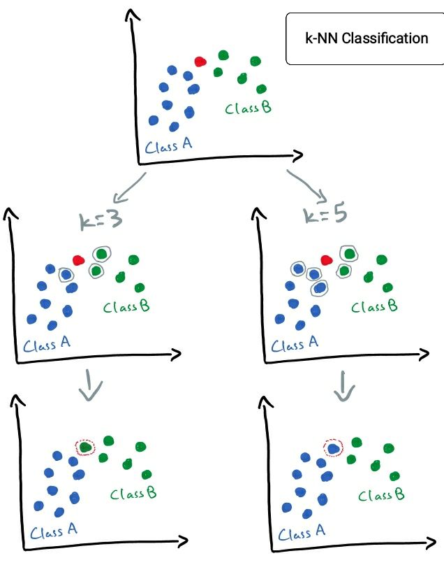
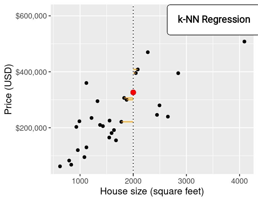
The k-NN algorithm works by finding the k data points in the training set that are closest in distance (e.g. Euclidean, Manhattan, Cosine) to the new data point, and then assigning the new data point to the class that is most common among its k nearest neighbors in classification tasks or predicting the target value of the new data point based on the average of the target values of its k nearest neighbors in regression tasks. The value of k is a user-defined parameter that controls the number of neighbors considered for classification or regression.

💡 Why is it useful?

The k-NN algorithm is easy to understand and implement, making it a popular choice for beginners in machine learning. Since the k-NN algorithm has no assumptions about the underlying distribution of the data, it can be used for a wide range of data types and structures.

👨‍💻 My personal story

When I first started learning machine learning, the k-NN algorithm was one of the first algorithms I encountered. I remember feeling intimidated by some of the more complex algorithms, but k-NN seemed simple and intuitive. I used it to classify handwritten digits in the MNIST dataset and was impressed by its accuracy and speed. As I continued to study machine learning, I’ve moved on to more advanced techniques (e.g. Neural Networks). However, I still appreciate the simplicity and versatility of k-NN.

📚 Who should learn it?

The k-NN algorithm is a useful tool to have for anyone learning AI. It can help you -as it helped me personally- to understand later on even more complex and powerful AI algorithms and be a better machine learning engineer.

🗣️ Let’s talk!

Do you have any experience using the k-NN algorithm? What applications have you used it for? If anyone would like to know more or has questions, feel free to ask in the comments below.

Below are my personal thoughts and reflections on Andrew Ng’s Stanford Machine Learning lecture on Generalized Linear Models (GLMs), including the key ideas I found interesting and how I understood them.

There is something that feels almost like magic in the mathematics of GLMs.

By changing only the underlying assumed probability distribution of the hypothesis function, and expressing it in the form of an exponential family distribution, we can derive several well-known machine learning algorithms:

  • Ordinary Least Squares, using the Gaussian distribution
  • Logistic Regression, using the Bernoulli distribution
  • Softmax Regression, using the Multinomial distribution

This is a beautiful mathematical abstraction. We can essentially plug in a different probability distribution and derive a corresponding model. For example, the Gamma or Poisson distributions.

What makes this even more interesting is that these machine learning algorithms are quite different from one another. Each solves a different type of problem: regression, binary classification, or multiclass classification.

And yet, they can all be understood through the same underlying mathematical framework.

Isn’t that awesome?

The GLMs can be derived from the probabilistic interpretation of these machine learning algorithms. Once we have that probabilistic foundation, typical gradient descent or gradient ascent can be used to minimize the loss function J(x, y, θ) or maximize the log-likelihood, log(L(θ)), when fitting a GLM to a dataset.

There is another aspect I find particularly fascinating.

From the probabilistic interpretation of these regression and classification algorithms, the logistic function emerges naturally from the mathematics. It isn’t simply an arbitrary function that happens to work well. The probabilistic formulation helps answer the deeper “why?” behind its use.

And that is what makes GLMs so beautiful to me.

Different algorithms. Different probability distributions. Different problems.

Yet one elegant mathematical framework connects them all.

This is magic.