Machine Learning friends! 💡
Let’s study something interesting! 📚
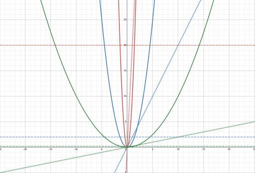
In this Desmos graph 📈, I would like to explain how the inverse of the second derivative of a loss function, (1 ÷ f”(x)), could be used as an initial estimate of the learning rate (α) when training ML models using gradient descent.
In the example, we have 3 simple convex quadratic functions (f(x)), (g(x)) and (h(x)) as solid lines (blue, red and green). Their first derivatives are the dotted lines, while their second derivatives (f”(x)), (g”(x)) and (h”(x)) are the dashed horizontal lines.
The second derivative tells us how quickly the first derivative changes. In our example:
So, the higher the curvature, the smaller the learning rate, and vice versa.
Higher curvature → smaller learning rate
Lower curvature → larger learning rate
This gives us a simple intuition for how the curvature of a loss function can help us choose an initial learning rate for gradient descent. 🚀